How can we tell what programming languages and technologies are used by the most people? How about what languages are growing and which are shrinking, so that we can tell which are most worth investing time in?
One excellent source of data is Stack Overflow, a programming question and answer site with more than 16 million questions on programming topics. By measuring the number of questions about each technology, we can get an approximate sense of how many people are using it. We’re going to use open data from the Stack Exchange Data Explorer to examine the relative popularity of languages like R, Python, Java and Javascript have changed over time.
Each Stack Overflow question has a tag, which marks a question to describe its topic or technology. For instance, there’s a tag for languages like R or Python, and for packages like ggplot2 or pandas.
1. Load the Libraries and DataSet
# Load libraries
library(tidyverse)      #  Loads all the tidyverse oackages
library(printr)         #  helps print better
library(patchwork)      #  grouping graphs together


# Load dataset
by_tag_year <- readr::read_csv("https://raw.githubusercontent.com/tagasimon/Evolution-of-Programming-Languages/master/datasets/by_tag_year.csv") # Read the csv using the readr package

# Inspect the dataset
head(by_tag_year) # prints the top 6 observations of the dataset| year | tag | number | year_total |
|---|---|---|---|
| 2008 | .htaccess | 54 | 58390 |
| 2008 | .net | 5910 | 58390 |
| 2008 | .net-2.0 | 289 | 58390 |
| 2008 | .net-3.5 | 319 | 58390 |
| 2008 | .net-4.0 | 6 | 58390 |
| 2008 | .net-assembly | 3 | 58390 |
2. Now in fraction format
This data has one observation for each pair of a tag and a year, showing the number of questions asked in that tag in that year and the total number of questions asked in that year. For instance, there were 54 questions asked about the .htaccess tag in 2008, out of a total of 58390 questions in that year.
Rather than just the counts, we’re probably interested in a percentage: the fraction of questions that year that have that tag. So Let’s visualize the top 12
by_tag_year %>%
        group_by(year, tag) %>%
        summarise(percent = number / year_total) %>%
        filter(year == 2008) %>%
        arrange(desc(percent)) %>%
        mutate(tag = fct_reorder(tag, percent)) %>%
        head(12) %>%
        ggplot(aes(tag, percent, fill = tag)) +
        geom_col(show.legend = FALSE) +
        coord_flip() +
        scale_y_continuous(labels = scales::percent_format(accuracy = 1)) +
        labs(x = "Tags",
             y = "Percentage of Search",
             title = "2008 StackoverFlow Search Tags",
             subtitle = "Top 12 Tags")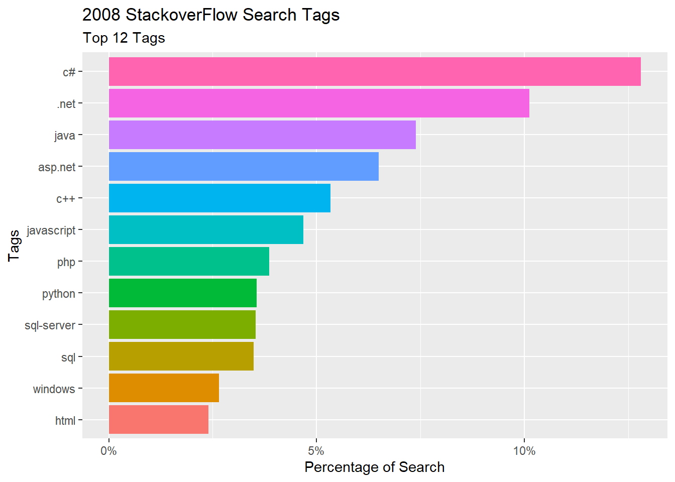
3. Has R been growing or shrinking?
Since we are Using R programming language. Wouldn’t we like to be sure it’s a good investment for the future? Has it been keeping pace with other languages, or have people been switching out of it?
Let’s look at whether the fraction of Stack Overflow questions that are about R has been increasing or decreasing over time.
Rather than looking at the results in a table, we often want to create a visualization. Change over time is usually visualized with a line plot.
by_tag_year %>%
        filter(tag == "r") %>%
        group_by(year) %>%
        summarise(percent = number / year_total) %>%
        ggplot(aes(as.factor(year), percent, group=1)) + # base ggplot2 function for plotting
        geom_point() + # scatter plot points
        geom_line() + # line plot
        scale_y_continuous(labels = scales::percent_format()) + # default scales for the y axis with percent labels
        labs(x = "Year",
             y = "% of the Total Searches",
             title = "Search Trend for R over the Years")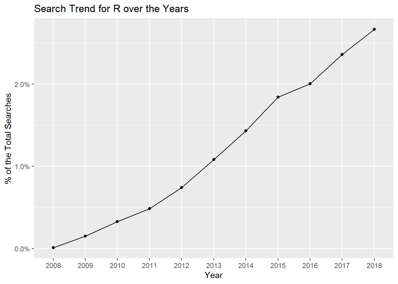
5. How about the Tidyverse Packages
Based on that graph, it looks like R has been growing pretty fast in the last decade. Good thing we’re practicing it now!
Besides R, we can look at the other tidyverse packages that have tags, we’ve already used some of them in this analysis.
Instead of just looking at R, let’s look at all three tags and their change over time. Are each of those tags increasing as a fraction of overall questions? Are any of them decreasing or Increasing?
tidy_tags <- tidyverse_packages() ## These are the tidyverse tags

by_tag_year %>%
        filter(tag %in% tidy_tags) %>%
        group_by(year, tag) %>%
        summarise(percent = number / year_total) %>%
        ggplot(aes(year, percent, color = tag)) +
        geom_point() +
        geom_line() +
        scale_y_continuous(labels = scales::percent_format())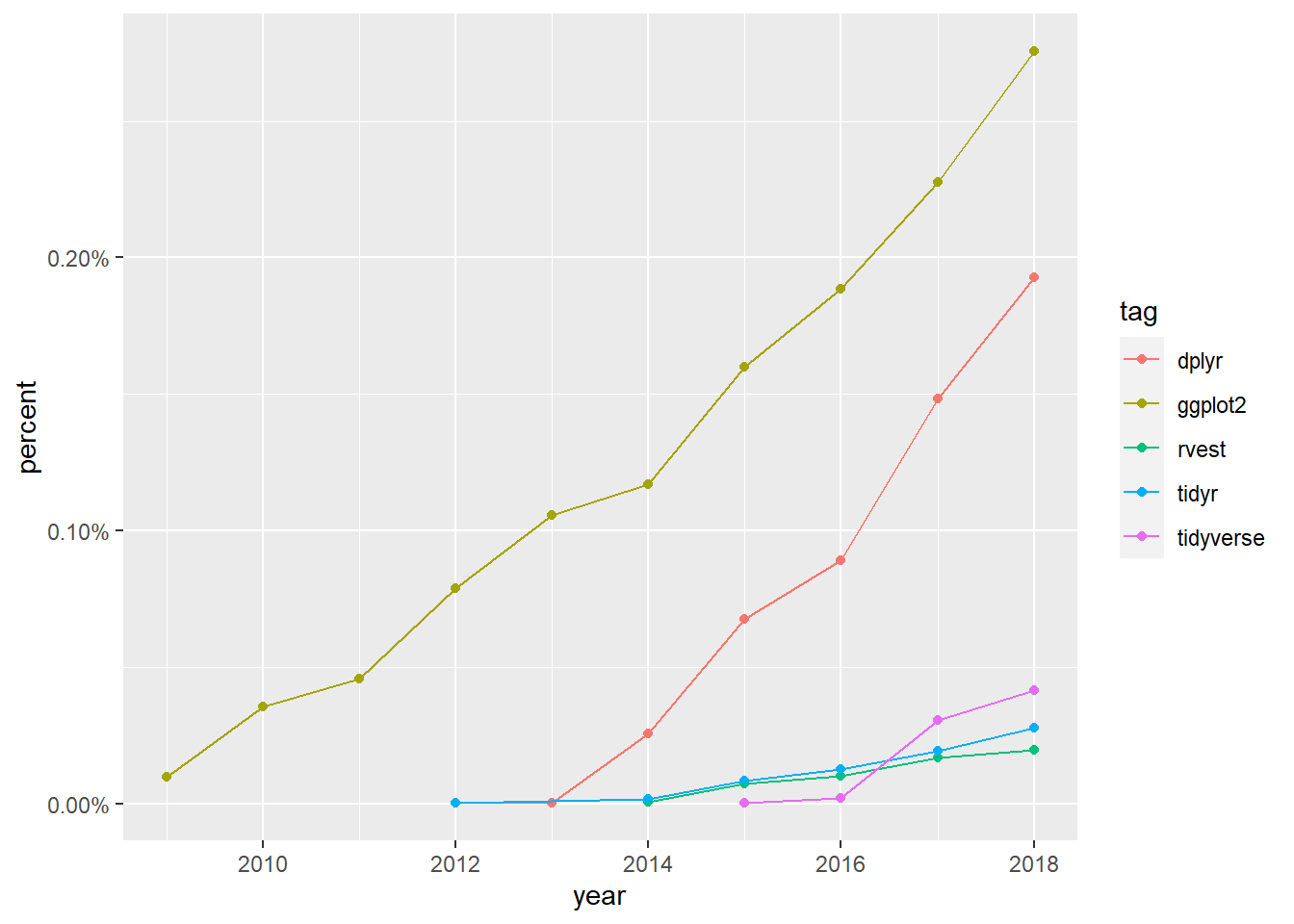
        labs(x = "Year",
             y = "% of the Total Searches",
             title = "Growth of R over the Years")
## $x
## [1] "Year"
##
## $y
## [1] "% of the Total Searches"
##
## $title
## [1] "Growth of R over the Years"
##
## attr(,"class")
## [1] "labels"6. What are the most asked-about tags?
It’s sure been fun to visualize and compare tags over time. The dplyr and ggplot2 tags are both growing quickly as well.
We might like to know which tags have the most questions overall, not just within a particular year. Right now, we have several rows for every tag, but we’ll be combining them into one. That means we want group_by() and summarize().
Let’s look at tags that have the most questions in history.
# head(by_tag_year)
by_tag_year %>%
        group_by(tag) %>%
        summarise(total = sum(number)) %>%
        arrange(desc(total)) %>%
        head(10) %>%
        mutate(tag = fct_reorder(tag, total)) %>%
        ggplot(aes(tag, total, fill = tag)) +
        geom_col(show.legend = FALSE) +
        coord_flip()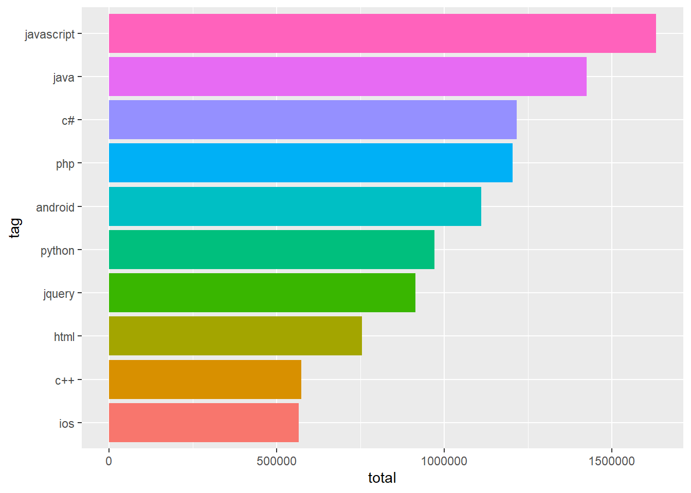
7. How have large programming languages changed over time?
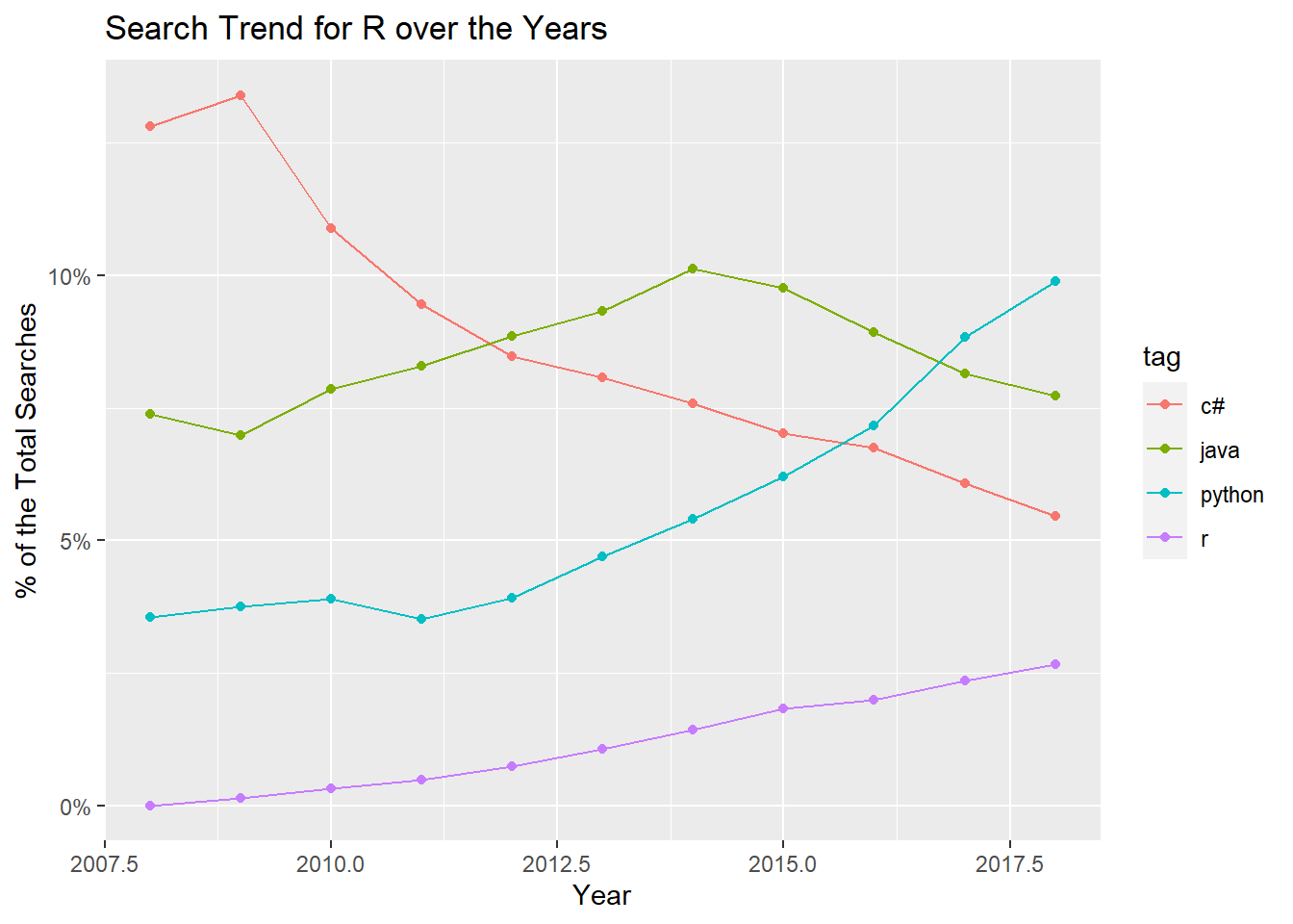
We’ve looked at selected tags like R, ggplot2, and dplyr, and seen that they’re each growing. What tags might be shrinking? A good place to start is to plot the tags that we just saw that were the most-asked about of all time, including JavaScript, Java and C#.
by_tag_year %>%
        filter(tag %in% c("python", "java", "c#", "r")) %>%
        group_by(year, tag) %>%
        summarise(percent = number / year_total) %>%
        ggplot(aes(year, percent, color = tag)) + # base ggplot2 function for plotting
        geom_point() + # scatter plot points
        geom_line() + # line plot
        scale_y_continuous(labels = scales::percent_format(accuracy = 1)) +
        labs(x = "Year",
             y = "% of the Total Searches",
             title = "Search Trend for R over the Years")